
Modeling a Gas Engine with Thermolib
The importance of self-sustaining energy supplies increases more and more. Therefore, it is common practice to combine a conventional engine with a battery and or reuse waste heat. This example will show how to model a gas engine with Thermolib. So, what’s the fuss? At a top level the engine is not a steady-state process and takes place in a closed volume. This bears some pitfalls, which we aim to tackle.
Contents
- Define Engine Inputs, Outputs and Parameters
- Determine Intake State
- Model Compression
- Calculate Combustion and Expansion
- Average Outputs over Cycle Time
- Conclusion
1. Define Engine Inputs, Outputs and Parameters
An engine needs a fuel and air to work. So these are our first two inputs. Also, the rotational speed is normally given externally by the balance of forces, depending on the clutch, the gear transmission and the travelling speed. Though the balance of forces is not subject of this example, these physical relations bear a first conflict. If we’re supplying a fuel and air flow, how can the rotational speed also be given, when the following applies
![]()
Where ![]() is the engine displacement,
is the engine displacement, ![]() the rotational speed and
the rotational speed and ![]() the number of strokes per cycle (i.e. a 4-stroke or 2-stroke engine). It is obvious this equation is fully determined by our inputs and the engine specific parameters. Or is it? In Thermolib a flow is defined by its mass flow. The equation above only defines a volume flow. The connecting state variable is the density, which for gases is mainly determined by the pressure. With given states of air and fuel the mass flow through the engine can be calculated. Only the input state is considered by the engine model. To find out more about the functional chain of pressure and flow in Simulink watch the webinar “What’s new in Release 5.2”.
the number of strokes per cycle (i.e. a 4-stroke or 2-stroke engine). It is obvious this equation is fully determined by our inputs and the engine specific parameters. Or is it? In Thermolib a flow is defined by its mass flow. The equation above only defines a volume flow. The connecting state variable is the density, which for gases is mainly determined by the pressure. With given states of air and fuel the mass flow through the engine can be calculated. Only the input state is considered by the engine model. To find out more about the functional chain of pressure and flow in Simulink watch the webinar “What’s new in Release 5.2”.
Obvious outputs of the engine model should be torque, exhaust gas and engine temperature. Other parameters needed for calculation are the compression ratio and the polytropic coefficient used for the model of compression and expansion (see Step 3).
An engine process is generally divided into the phases:
- Intake
- Compression
- Combustion and Expansion
- Exhaust
In our model the state of the intake is given and the states after the other stages need to be calculated as described in the following steps.
2. Determine Intake State
First of all we need to figure out how to use the Thermolib concept of the FlowBus with a discrete quantity. As the name suggests the bus structure is designed to describe flows. It is likewise usable with quantities, though. Internally Thermolib calculates specific state variables (i.e. enthalpy in J/mol) and later multiplies these with the mass flow. The unit of the mass flow signal “ndot” on the bus is thought to be in amount per time (i.e. mol/s). But this is merely a convention, though a sensible one. As the information of the unit is not stored within the bus or signal, it is open for interpretation. This approach is not disturbing the function of other blocks, as long as the units are consistent.
The examples above show that the signal “ndot” may be interpreted as a quantity and subsequently the states are specific to the same. This will be used in the following to calculate the engine cycle with a fixed enclosed mass.
The properties at the intake are given by the input flows and the volume of the engine by the compression ratio and engine displacement. Thus, the mass contained within the engine per cycle can be calculated.
![]()
With compression ratio ![]() defined as
defined as
3. Model Compression
Compression and expansion can be modelled by the polytropic equation:
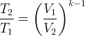

Where ![]() is the polytropic coefficient. As the compression ratio is known and constant, the temperature after compression or expansion can be calculated. With the mass and volume known, the density may be derived. With the “T-rho State” block the complete state can now be calculated.
is the polytropic coefficient. As the compression ratio is known and constant, the temperature after compression or expansion can be calculated. With the mass and volume known, the density may be derived. With the “T-rho State” block the complete state can now be calculated.
With the following fundamental equation the work is determined. For simplicity the cylinders are modeled adiabatically.
![]() With inner energy
With inner energy ![]() defined as
defined as
4. Calculate Combustion and Expansion
Use the “Reactor” block to calculate the combustion after the compression. You can reuse the block created for compression with inverse compression ratio.

5. Average Outputs over Cycle Time
The total work done in one cycle is
![]()
The average power of the current time step may be estimated analogously to the first equation with
![]()
The same holds for the mass flow.
6. Conclusion
The complete model is shown below. It is of course kept simple yet it can be easily expanded to account for
- heat losses and cooling,
- inertia of the engine or
- direct injection.
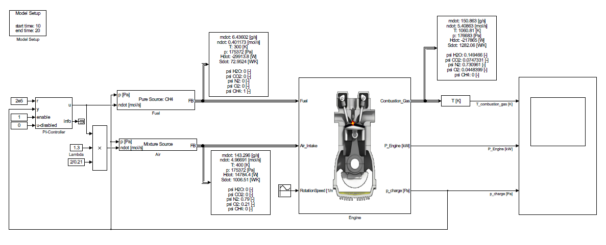

You can download the model file. We also supply an extended version, which already accounts for heat losses. So have a look. Now, it’s your turn. We’re looking forward to your comments!
